
Copy of Skull Stripping / Brain Diffusion Pipeline Protocall
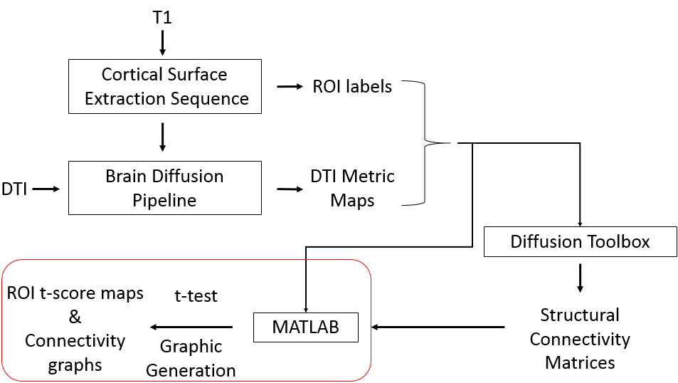
DTI Metrics and DTI-based Structural Connectivity for ROI Analysis
Below is an overview of the processing pipeline.

To begin, T1 and diffusion tensor imaging (DTI) sequence will need to be acquired. Magnetic resonance imaging (MRI) sequence are acquire and saved in Digital Imaging and Communications in Medicine (DICOM) format (.dcm extension). These files will need to be converted into Neuroimaging Informatics Technology Initiative (NIfTI) files (.nii extension). Software such as MRIcron (www.mccauslandcenter.sc.edu/crnl/mricron/) or MRIconverter can be utilized to perform this task.
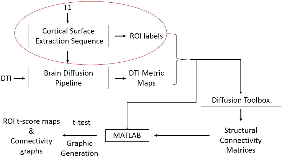
The T1 sequence will be used to segment the brain into different components (i.e. white matter (WM), gray matter (GM), and specific regions of interest (ROIs)). In this protocol, we will use BrainSuite to segment the brain into different ROIs. BrainSuite comes with default atlases such as BrainSuite_atlas1. For our study, we imported an atlas from CONN-fMRI Functional Connectivity toolbox (www.nitric.org/projects/conn), which contained Brodmann areas from the Talairach Daemon atlas (www.talairach.org) along with four Fox ROIs that were brought into MNI-space through a Lancaster transform. The process of creating a custom atlas within BrainSuite can be found here:
http://brainsuite.org/processing/svreg/creating-custom-atlases/
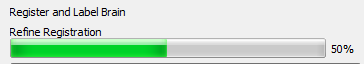
BrainSuite segments the brain images through a cortical surface extraction sequence, which begins with skull-stripping. Following this, the program will go through several stages including, “Skull and scalp”, “Nonuniformity correction”, “Tissue classification”, “Cerebrum labeling”, “Inner cortical mask”, “Scrub mask”, “Topology correction”, “Wisp removal”, “Inner cortical surface”, “Pial surface”, “Split hemispheres”, and finally “Register and label brain”. At this final stage, BrainSuite will perform a surface volume registration (svREG) that involves warping a ROI labelled atlas into the form of an individual subject’s brain. BrainSuite saves output files at each stage of processing. Here we will be interested in the bias field corrected T1 image sequence (This will be used in the Brain Diffusion Pipeline) and the ROI labels (This will be used by custom MATLAB scripts for t-score maps and ROI-specific DTI metrics. This will also be used by BrainSuite to find structural connectivity at specific ROIs.) for each subject analyzed. The procedure below goes through the methodology of processing these T1 image sequences with BrainSuite.
Cortical Surface Extraction Sequence: Skull stripping and labelling
Open the T1 sequence in NIfTI format
Cortex>Skull Stripping (BSE)
For BrainSuite17A uncheck “automate parameters selection”
Deselect “trim spinal cord/brain stem”.
Click “Step” four times (5 times for 17A) and inspect the mask on the axial image of the brain. (To view different slices, hover mouse cursor over the image and scroll up or down). Click “Back” four times to remove mask.
If needed, Adjust Diffusion Iterations, Diffusion Constant, Edge Constant, and Erosion Size as needed until the mask is aligned with the brain on all slices. (Ensure no gaps and abnormalities are within the mask). Start adjustments with the Edge Constant (The higher the smaller ROI is created). If that does not work, try adjusting the Diffusion constant (the greater, the smoother image becomes).
If the mask is still not satisfactory or needs a few manual touch ups, check “edit mask”

within the Delineation Toolbox under the Mask Tool. Now you can manually edit the manual by Ctrl + Right Click to add and Ctrl + Left Click to subtract.
Once mask is satisfactory, Save the mask as “SubjectID_mask.nii” Cortex>Cortical Surface Extraction Sequence
Uncheck “Skull Stripping”
Check “Register and label brain”
Select “CustomAtlas” (“MNIAtlas” on some computers) in the Labeled Atlas dropdown box
Then click “Run All”
For “CustomAtlas”, an error should occur at 50%.

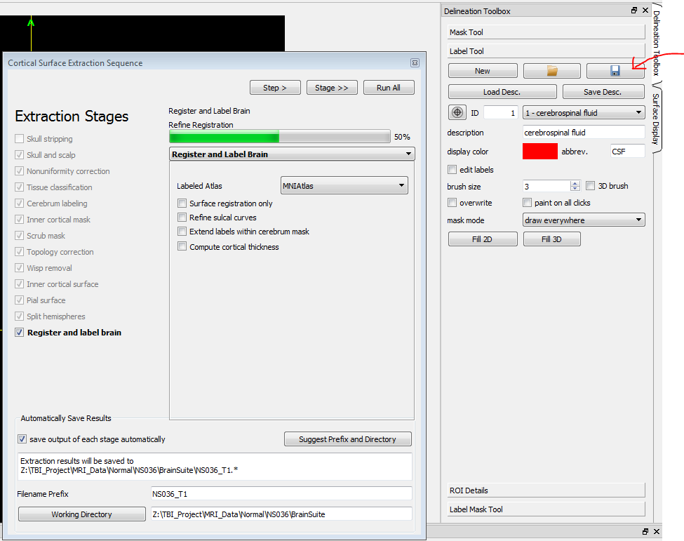
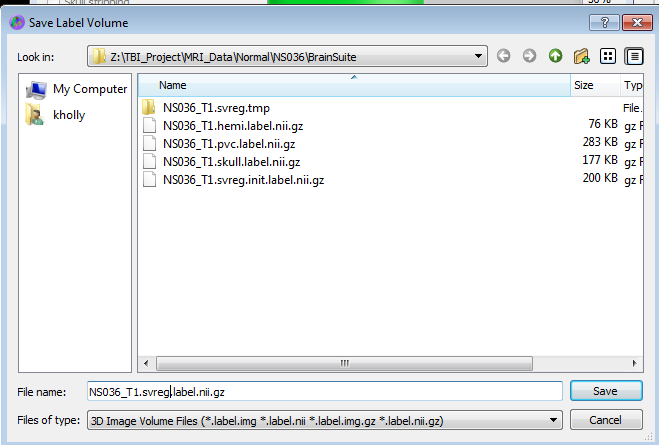
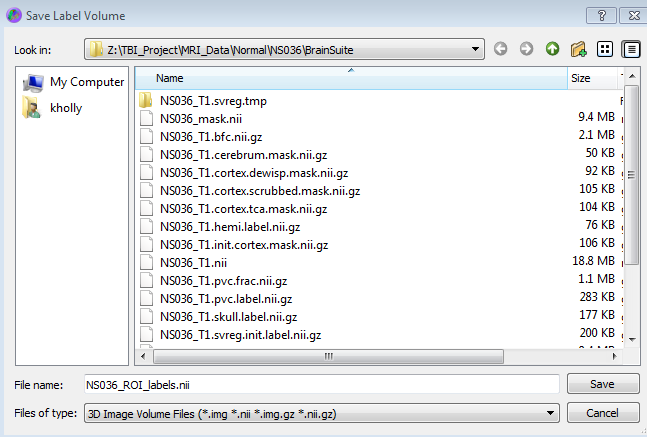
At this point, the label should be saved as “SubjectID.svreg.label.nii.gz”. Labels without the description can be saved as “SubjectID_ROI_labels.nii” by selecting “.img .nii” in the dropdown box when saving.
This process creates the ROI label file (SubjectID.svreg.label.nii.gz) and the bias field corrected T1 image sequence (SubjectID_T1.bfc.nii.gz) that will be needed later. The cortical thickness can be found in txt file called “SubjectID.roiwise.stats” under the heading ‘Mean thickness’. Although it acquires the cortical thickness with the default atlas’s ROIs.
Save ROI labels[HKS1] as (.nii and not .nii.gz)
[HKS1]describe

BDP (Brainsuite Diffusion Pipeline) to obtain diffusion tensor
Open the Windows command prompt.
Click “Start” on the taskbar and type “cmd” in the search bar.
Type the following command in the command window:
"C:\Program Files\BrainSuite15c\bdp\bdp.exe" subjectID_T1.bfc.nii.gz --FRT --FRACT --tensor --nii subjectID.dwi.nii.gz -g subjectID.bvec -b subjectID.bval
Or
"C:\Program Files\BrainSuite16a\bdp\bdp.exe" subjectID_T1.bfc.nii.gz --FRT --FRACT --tensor --nii subjectID.dwi.nii.gz -g subjectID.bvec -b subjectID.bval
Note: You may need to type the file location for each file.
Once the program is done running, you will have the following files:
SubjectID.dwi.RAS.correct.T1_coord.eig.nii
SubjectID.dwi.RAS.correct.SH.FRT.T1_coord.odf (Located in FRT folder)
SubjectID.dwi.RAS.correct.SH.FRACT.T1_coord.odf (Located in FRACT folder)
The DTI metrics maps included fractional anisotropy (FA), mean diffusivity (MD), axial diffusivity (AD), radial diffusivity (RD), mean apparent diffusion coefficient (mADC), L2, and L3
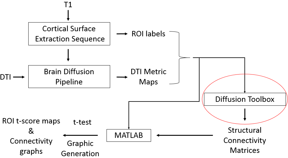
Using BrainSuite to find Connectivity (DTI based)
Open up BrainSuite
File > Open Volume… Load SubjectID.dwi.RAS.correct.T1_coord.eig.nii
The Diffusion Toolbox should open when file is opened.
Click on the “Tractography” tab in the Diffusion toolbox to open it. When using diffusion tensors to create tracks, make sure that “compute from DTI” is checked.
Enter project’s specified parameters.
Epilepsy, MS, and mTBI
2 seed/voxel
10 mm
500 steps
35 degrees
0.2 FA
PD and MTS
2 seed/voxel
25 mm
250 steps
45 degrees
0.2 FA
Click “Compute Tracks” to produce the fiber tracks.
Go to File > Open > Label Volume… SubjectID.svreg.label.nii.gz
Open the “Connectivity” tab of the Diffusion toolbox
Uncheck merge GM and WM ROIs in cortical labels
Click “Compute Connectivity.” After a few moments of calculation, a circle graph will appear, displaying connectivity between all brain regions.
Go to File > Save Connectivity Matrix
Save files as “SubjectID_SCM”.
DTI Metrics
Create Directory with the following folders:
Mask, Labels, FA, MD, RD, AD, mADC, L2, and L3
Filenames within respective folders:
SubjectID_mask.nii
SubjectID_ROI_labels.nii
SubjectID.dwi.RAS.correct.FA.T1_coord.nii.gz
SubjectID.dwi.RAS.correct.MD.T1_coord.nii.gz
SubjectID.dwi.RAS.correct.RD.T1_coord.nii.gz
SubjectID.dwi.RAS.correct.AD.T1_coord.nii.gz
SubjectID.dwi.RAS.correct.mADC.T1_coord.nii.gz
SubjectID.dwi.RAS.correct.L2.T1_coord.nii.gz
SubjectID.dwi.RAS.correct.L3.T1_coord.nii.gz
MATLAB scripts:
DTI_ROI_analysis.m
tscore_atlas_fig.m
Structural Connectivity
Create Directory with the following folders:
mTBI and Norm
Filenames within respective folders:
SubjectID_CM_unrefined
MATLAB scripts:
circulargraphforCM_MNI_unrefined.m
redblueconnectivitygraph.m
circulargraphforCM_MNI_unrefined_sumrow.m
Connectome.m